Applications of Marine Magnetometers and Gradiometers: The Instrument That Sees Iron, Not Shape

Every instrument covered so far in this series — side-scan sonar, sub-bottom profiler, multibeam and single-beam echosounders — works by sending sound into the water and listening for what comes back. A marine magnetometer does neither. It sends nothing at all. It simply listens, passively, to tiny distortions in the Earth's own magnetic field, distortions that reveal one thing very well: the presence of iron and steel, buried or not, regardless of what shape it happens to be.

How Marine Magnetometers and Gradiometers Work

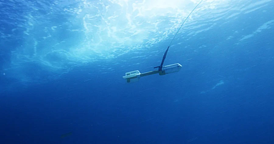
A total-field magnetometer is a single instrument that records the strength of the ambient magnetic field at one location at a time, expressed in nanotesla. Iron and steel objects locally distort that field, creating a detectable magnetic anomaly. A gradiometer takes the same underlying measurement but arranges two or more sensors in a fixed configuration, calculating the difference between their readings — expressed in nT per meter rather than nT alone. That differencing step is what makes gradiometers valuable for shallow-target work: it suppresses slow, region-wide magnetic drift (including daily "diurnal" variation in the Earth's field) and long-wavelength geological effects, leaving the sharp, localized anomalies produced by nearby ferrous objects standing out far more clearly than they would in raw total-field data.

Sensor technology has advanced considerably since the field's origins. Fluxgate sensors remain lightweight and low-power but offer comparatively modest precision. Cesium vapor and Overhauser sensors, both now standard for marine work, are considerably more sensitive — a peer-reviewed evaluation of the Overhauser-type JOM-4S instrument found a sensitivity on the order of 0.01 nT, roughly an order of magnitude finer than a classical proton-precession magnetometer. A widely used marine cesium vapor system, the Geometrics G-882 (nicknamed "Magnetron" aboard USGS survey vessels), samples at up to 20 Hz with a heading error under 1 nT, is depth-rated to 4,000 psi, and is typically towed at a distance of roughly four times the survey vessel's length to keep the ship's own hull out of the reading.

A History Written in Magnetic Stripes

Marine magnetometry owes its existence to submarine warfare. Working at Gulf Research in the years leading up to 1940, physicist Victor Vacquier developed the fluxgate magnetometer, which the U.S. Navy adapted into an airborne magnetic anomaly detector (MAD) — a sensor typically mounted on a trailing boom or towed "stinger" to keep the aircraft's own metal fuselage from swamping the reading. Operational aircraft carrying Vacquier's instrument were already flying anti-submarine patrols near the British West Indies and Martinique by July 1942, and by 1943 magnetic anomaly detectors equipped most Allied anti-submarine patrol aircraft.

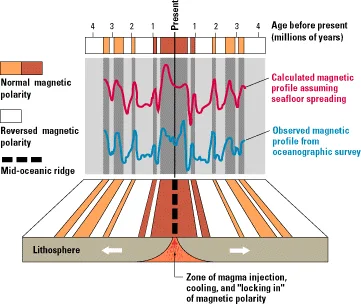
After the war, Vacquier — who later joined Scripps Institution of Oceanography — refitted his surplus fluxgate instruments to be towed behind research vessels instead of aircraft, opening an entirely new line of inquiry: what would the seafloor's own magnetism look like, mapped continuously across an ocean basin? What his surveys found across the Mendocino Fracture Zone was too strange to ignore — enormous lateral offsets in the magnetic pattern of the seafloor that hinted at large-scale horizontal motion no one had a framework to explain yet. Meanwhile, in 1954, Russell Varian and Martin Packard at Varian Associates invented the proton-precession magnetometer, an instrument that soon proved even better suited to continuous towed marine surveying. Naval Oceanographic Office survey ships used instruments like it through the late 1950s and early 1960s to compile systematic magnetic charts of the ocean floor, revealing a striking, zebra-like pattern of alternating magnetic polarity utterly unlike anything seen on land.

The explanation arrived in 1963. Frederick Vine and Drummond Matthews in Cambridge — and, independently, Canadian geophysicist Lawrence Morley — proposed that newly formed seafloor rock locks in the direction of Earth's magnetic field at the moment it solidifies at a mid-ocean ridge. As the field itself periodically reverses polarity over geological time, and as new crust keeps spreading outward from the ridge in both directions, the seafloor records that history as parallel, mirror-image stripes of alternating polarity. Marine magnetometer profiles across ridges like the East Pacific Rise matched the independently established timeline of magnetic reversals so precisely that the Vine–Matthews–Morley hypothesis became one of the decisive pieces of evidence for seafloor spreading — and, by extension, for plate tectonics itself.

Total Field or Gradient? Choosing the Right Setup

Marine magnetometers have supported seismic survey vessels as a low-cost companion instrument since the 1950s, and a single total-field sensor remains entirely adequate for wide-area reconnaissance — regional geological mapping, crustal structure studies, and broad tectonic surveys where the target of interest is a large, deep, or gradual magnetic feature rather than a compact object sitting close to the sensor. Gradiometer arrays earn their added cost and complexity specifically where the opposite is true: shallow, discrete, human-scale ferrous targets that would otherwise be masked by diurnal drift or regional geological "noise" in a single-sensor reading. That trade-off — simplicity and area coverage on one side, precision and target discrimination on the other — is what determines which configuration a given survey actually needs.

Core Applications in the Field

UXO detection and offshore wind or cable clearance

Unexploded ordnance surveys are the application where gradiometer precision matters most directly for safety. A 2005 U.S. Geological Survey field test at the Standardized UXO Test Site in Yuma Proving Ground demonstrated a prototype tensor gradiometer — a 1-meter tetrahedral array of four triaxial fluxgate sensors known as TESSA — successfully producing a sharp, well-centered anomaly over a 60-mm mortar shell buried just 0.25 m deep, surveyed on a tight 0.25-m grid. Offshore, this same gradient-sensing principle underlies pre-installation UXO surveys for wind farm foundations and cable routes, typically run alongside side-scan sonar and sub-bottom profilers as a combined instrument suite; guidance published by the Carbon Trust in April 2020 codifies best practice for exactly this kind of combined geophysical UXO and boulder survey ahead of offshore cable installation.

Pipeline and submarine cable route detection

Because steel pipelines and armored submarine cables are themselves strongly magnetic, a magnetometer or gradiometer can locate and verify their position even once they are buried, without needing to expose them. Published depth-estimation techniques — including a tilt-angle method described in the Journal of Pipeline Systems Engineering and Practice, where a 90° tilt angle in the magnetic field marks a pipeline's exact location and the offset to the adjacent 0° point yields its burial depth — turn a magnetic anomaly profile directly into a location-and-depth estimate. More recent research pushes this further: a 2024 study in the Journal of Geophysics and Engineering trained an end-to-end neural network on 140,000 synthetic magnetic anomaly samples to map submarine cable positions directly, achieving 99.935% classification accuracy and horizontal position errors under 0.5 m in testing — a substantial improvement over traditional inversion methods for this kind of route verification work.

Maritime archaeology and shipwreck detection

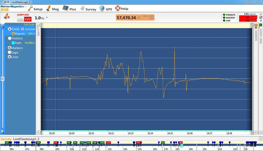
Because a wooden shipwreck can be acoustically invisible once it has broken down or become buried in sediment, its iron fittings, anchors, engines, and cargo often remain the most reliable way to find it magnetically, long after side-scan sonar has stopped showing anything of interest. A single, isolated anomaly in a magnetometer readout typically indicates a small, discrete object, while a cluster of anomalies grouped together points to a larger mass of material — exactly the kind of signature archaeologists use to distinguish a stray piece of debris from an actual wreck site. Magnetic prospecting has a long academic pedigree in archaeology on land as well: the method's first documented archaeological application dates to 1958 in England, using an early proton magnetometer, and it has since become one of the most widely used non-invasive tools for locating buried remains, on land and underwater alike.

Regional geological and tectonic mapping

The application that started it all has never gone away: marine magnetic surveys remain a standard, low-cost companion to seismic reflection data for interpreting crustal structure, and the same magnetic-striping principle that helped confirm seafloor spreading in the 1960s continues to inform how geologists read the age and history of oceanic crust today.

Conclusion

From a submarine-hunting sensor bolted to a WWII patrol plane, to the instrument that produced arguably the single most convincing piece of evidence for plate tectonics, to a routine line item on a modern offshore wind UXO survey — the marine magnetometer and its gradiometer variant have quietly done one job exceptionally well for nearly a century: finding iron and steel that acoustic instruments either cannot see or were never built to look for in the first place.

References

1. Wold, R.J., Cooper, A.K. (1989) — Marine magnetic gradiometer: A tool for the seismic interpreter, Geophysics
2. Liu, Y., Wu, Y., Li, G., Abbas, A., Shi, T. (2024) — Submarine cable detection using an end-to-end neural network-based magnetic data inversion, Journal of Geophysics and Engineering
3. Bracken, R.E., Brown, P.J. (2005) — Reducing Tensor Magnetic Gradiometer Data for Unexploded Ordnance Detection, USGS Scientific Investigations Report 2005-5046
4. Herbich, T. (2015) — Magnetic prospecting in archaeological research: a historical outline, Archaeologia Polona, Vol. 53
5. Gong, X., Chen, S., Zhang, S. (2021) — JOM-4S Overhauser Magnetometer and Sensitivity Estimation, Sensors
6. ASCE — Determining the Depth and Location of Buried Pipeline by Magnetometer Survey, Journal of Pipeline Systems Engineering and Practice, Vol. 11, No. 2
7. Wikipedia — Victor Vacquier; Magnetic anomaly detector; Vine–Matthews–Morley hypothesis
8. USGS — This Dynamic Earth: Magnetic Stripes and Isotopic Clocks; Geometrics G-882 Magnetometer
9. NOAA Ocean Exploration — Magnetometer
10. US EPA — Waterborne Magnetic Surveying
11. Applied Acoustics — What are UXO Surveys?
12. Carbon Trust — Guidance for Geophysical Surveying for Unexploded Ordnance and Boulders Supporting Cable Installation (April 2020)